Uniform flow around a circle

A brief description of the mathematics behind the scene

Velocity field and the stream function in two dimensions

If we have a (steady-state) incompressible, nonviscous fluid in two dimensions, we are interested in finding its velocity field $$\mathbf V = \left(u(x,y), v(x,y)\right).$$ From vector analysis we know that the stream function $\psi$ must satisfy \begin{eqnarray}\label{cond1} u=\frac{\partial \psi}{\partial y},\quad v=-\frac{\partial \psi}{\partial x}. \end{eqnarray}

Knowing this, consider the stream function $$\psi = Uy\left(1- \frac{a^2}{x^2+y^2} \right)$$ The level curves $\psi = \text{const}$ are called streamlines of the flow and they follow the direction of the velocity field, see figure below.

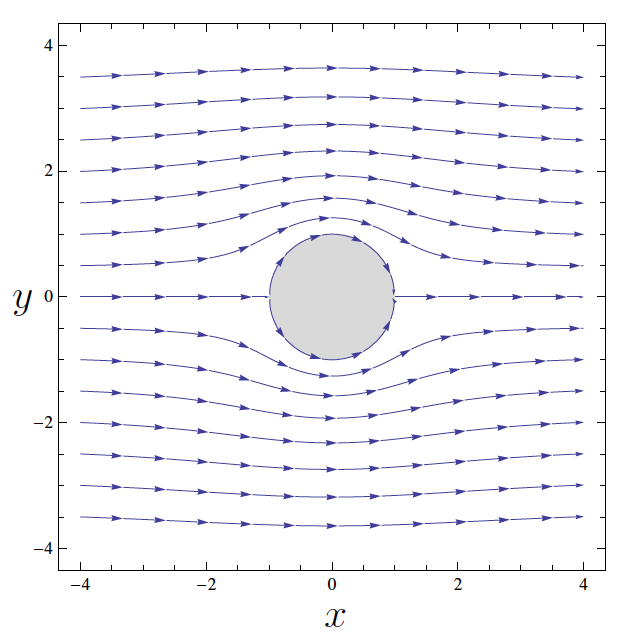
Streamlines $\psi= \text{const}$ with $U>0$ and $a=1$.

In this case, from (\ref{cond1}), the components of the velocity field $\mathbf V$ are \begin{eqnarray}\label{vel1} u = U\left(1 - a^2\frac{x^2-y^2}{(x^2+y^2)^2}\right),\qquad v= -2 U^{2} a^{2} \frac{ x y}{ \left(x^{2} + y^{2} \right)^{2}}. \end{eqnarray} This field represents a uniform flow around a circle of radius $a$ with center at $(0,0)$ and speed $U$, in the $x$-direction.

Simulation

For this simulation I used equations (\ref{vel1}) but considering a circle with center at $(x_0, y_0)$. Thus the components of the velocity field $\mathbf V $ are \begin{eqnarray*} u & = &U \left(1 - a^2\frac{(x-x_0)^2-(y-y_0)^2}{((x-x_0)^2+(y-y_0)^2)^2}\right),\\ v & = & -2 U^{2} a^{2} \frac{ (x-x_0) (y-y_0)}{ \left((x-x_0)^{2} + (y-y_0)^{2} \right)^{2}}. \end{eqnarray*}

Since the fluid particles move in accordance with the autonomous, first order system of ordinary differential equations \begin{eqnarray}\label{system} \dfrac{dx}{dt} = u, \quad \dfrac{dy}{dt} = v; \end{eqnarray} an individual particle's position $\mathbf x(t)= (x(t), y(t))$ is uniquely determined solely by its initial condition, that is, when $t=0$.

We can use numerical methods to approximate the solutions of system (\ref{system}). In particular, I used a 4th order Runge-Kutta method.

The source code of the simulation can be found in GitHub.

Uniform flow around a circle

Velocity field and the stream function in two dimensions

Simulation

Further reading