Multivariate Calculus
&
Ordinary Differential Equations
Lecture 4
1 Ordinary Differential Equations
1.3 Euler's Method for Solving ODEs Numerically
Stewart, Section 9.2 covers Euler's method.
The method gives a simple approximate solution to an ODE and is closely related to the notion of a slope field.
1 Ordinary Differential Equations
1.3.1 Euler's method using tangent lines
What is the equation of the straight line with slope $m$ that passes through the point $(t,y) = (a,b)$?
For any point $(t,y)$ on the line, we have
$\qquad \ds\frac{y-b}{t-a} = m $ $\Rightarrow\, y -b= m(t-a)$
$\;\qquad \qquad \qquad \Rightarrow \, y = m(t-a)+b.$
1 Ordinary Differential Equations
1.3.1 Euler's method using tangent lines
Euler's method uses tangent lines as approximations to solution curves. The tangent line to a solution curve of $y'=f(t,y)$ at $(t_0,y_0)$ is $$ y=y_0+f(t_0,y_0)(t-t_0). $$
This approximates the curve when $t$ is close to $t_0$.
1 Ordinary Differential Equations
1.3.1 Euler's method using tangent lines
Now imagine a family of solution curves to the differential equation. We can calculate an approximate value for $y$ at some later time by taking lots of small steps in time. At each step we will use the tangent line to the solution through our current point. This is Euler's method.
Using $\Delta t$ as the step size for our algorithm, let
$t_1=t_0+\Delta t,\; t_2=t_1+\Delta t,\qquad \;\,$
$t_3=t_2+\Delta t,\;\ldots\;,t_n=t_{n-1}+\Delta t.$
1 Ordinary Differential Equations
1.3.1 Euler's method using tangent lines
$t_1=t_0+\Delta t,\; t_2=t_1+\Delta\; t_3=t_2+\Delta t,\;\ldots\;,t_n=t_{n-1}+\Delta t.$
To find approximate $y$ values at these times, use the following equations in sequence:
$y_1=y_0+f(t_0,y_0)\Delta t $
$y_2 =y_1+f(t_1,y_1)\Delta t$
$y_3=y_2+f(t_2,y_2)\Delta t,$
and so on.
1 Ordinary Differential Equations
$t_1=t_0+\Delta t,\; t_2=t_1+\Delta\; t_3=t_2+\Delta t,\;\ldots\;,t_n=t_{n-1}+\Delta t.$
$y_1=y_0+f(t_0,y_0)\Delta t, \,$ $y_2 =y_1+f(t_1,y_1)\Delta t,\,$ $y_3=y_2+f(t_2,y_2)\Delta t,$ $\ldots$
1 Ordinary Differential Equations
1.3.1 Euler's method using tangent lines
Example: Use Euler's method with $\Delta t=0.2,$ to find an approximate solution to $y(0.6)$ for the IVP \[ \dif{y}{t}=2t,\qquad y(0)=0. \] Compare your answer with the actual value.
1 Ordinary Differential Equations
1.3.1 Euler's method using tangent lines
Example: Use Euler's method with $\Delta t=0.2,$ to find an approximate solution to $y(0.6)$ for the IVP $\,\ds\dif{y}{t}=2t,$ $y(0)=0.\,$ Compare your answer with the actual value.
Since $\frac{dy}{dt}=2t,\,$ $f(t,y)= 2t.$
| $n$ | $t_n$ | $y_n$ | $ f(t_n,y_n) $ | $ y_{n+1}$ $= y_n + f(t_n,y_n)\Delta t$ |
| $0$ | $0$ | $0$ | $2\times 0$$\,=0$ | $ 0+0\times 0.2 $ $=0$ |
| $1$ | $0.2$ | $0$ | $ 2\times 0.2$ $=0.4$ | $ 0+0.4\times 0.2$$\,=0.08$ |
| $2$ | $0.4$ | $0.08$ | $ 2\times 0.4=0.8$ | $ 0.08+0.8\times 0.2=0.24$ |
| $3$ | $0.6$ | $0.24$ | $ -$ | $ -$ |
1 Ordinary Differential Equations
1.3.1 Euler's method using tangent lines
Example: Use Euler's method with $\Delta t=0.2,$ to find an approximate solution to $y(0.6)$ for the IVP $\,\ds\dif{y}{t}=2t,$ $y(0)=0.\,$ Compare your answer with the actual value.
So with a stepsize of $0.2$ we have that $y(0.6) \approx 0.24$
To compute the exact value,
we know that $\ds \frac{dy}{dt} = 2t$
$\,\Ra\ds y = \int 2t dt$
$ =t^2 + C.$
For $y=0,\,$ then
$C = 0.$
So the exact solution is $y=t^2.$
Hence $y(0.6) = 0.36.$
The result we got with $\Delta t = 0.2$ is not very accurate.
The step size is too big! ☹️
1 Ordinary Differential Equations
1.3.1 Euler's method using tangent lines
The method is only accurate if you make $\Delta t$ small, which means a large number of steps is usually required. For this you might want to use Matlab. Define a $t$ vector and an initial $y$ value, then use the for command to iterate.
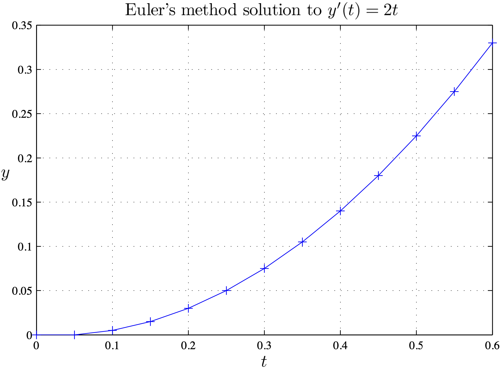
In the example $\Delta t=0.05$ and 12 steps have been chosen to take $t$ to $0.6$.
t = (0:0.05:0.6);
y(1) = 0;
for i = 1:12
  y(i+1) = y(i) + 2 * t(i) * 0.05;
end
y(13)
plot(t, y,'-')
1 Ordinary Differential Equations
1.3.1 Euler's method using tangent lines
1 Ordinary Differential Equations
1.3.1 Euler's method using tangent lines
Using Matlab we find $y(0.6)=0.33$ which is much much better than the previous estimate value for $y(0.6)$.
Note that we start with $y(1)=0,$ whereas in the theoretical work we write $y(0)=0$. Matlab does not allow you to put an index of zero. Keep this in mind in case you ever get the Matlab error message:
??? Index into matrix is negative or zero.
1 Ordinary Differential Equations
1.3.2 Euler's method using Matlab; an example
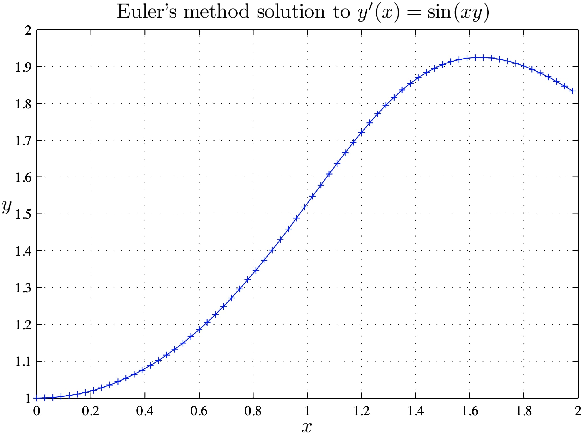
Consider the IVP $ \ds\dif{y}{x}=\sin(xy),\; y(0)=1.\, $ Matlab code to estimate $y(2),$ using Euler's method with step size $\Delta x=0.01$ is:
									x = (0:0.01:2);
									y(1) = 1;
									for i = 1:200
									  y(i+1) = y(i) + sin(x(i) * y(i)) * 0.01;
									end
									y(201)
									plot (x,y,'-')
Using Matlab we find $y(2)=1.8243.$
1 Ordinary Differential Equations
1.3.2 Euler's method using Matlab; an example
1 Ordinary Differential Equations
1.3.3 Demonstrating errors in Euler's method
Use Euler's method to approximate the solution curve of the initial value problem
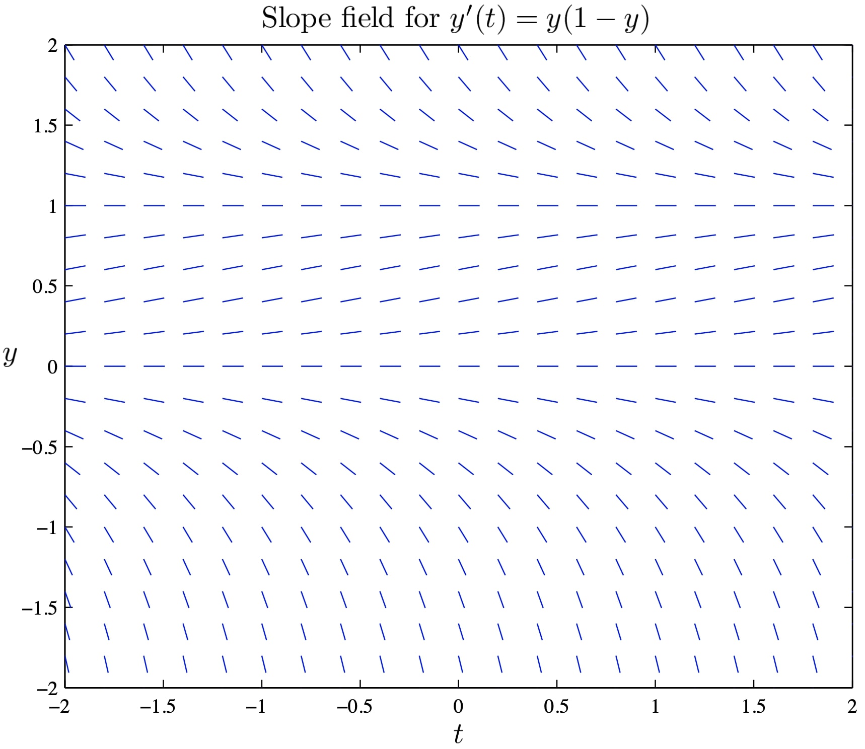
$y' = y(1-y),\quad y(-2) = 2.$
1 Ordinary Differential Equations
1.3.3 Demonstrating errors in Euler's method
Use Euler's method to approximate the solution curve of the initial value problem
$y' = y(1-y),\quad y(-2) = 2.$
Use the slope field below as a guide to draw in the approximate solution curve. What goes wrong in this case?
1 Ordinary Differential Equations
1.3.3 Demonstrating errors in Euler's method
Use Euler's method to approximate the solution curve of the initial value problem $ y' = y(1-y),\,$ $ y(-2) = 2. $ Use the slope field below as a guide to draw in the approximate solution curve. What goes wrong in this case?
1 Ordinary Differential Equations
1.3.4 Main points
- You should understand how slope fields lead to Euler's method.
- You should know how to approximate a solution to an IVP using Euler's method by hand.
- You should know how to implement Euler's method in Matlab.
- You should understand that errors can be a problem in the approximate solution, especially if a large step size is used.