Multivariate Calculus
&
Ordinary Differential Equations
Lecture 20
2 Functions of Several Variables
2.3 Contour diagrams
Geographical maps have curves of constant height above sea level, or curves of constant air pressure (isobars), or curves of constant temperature (isothermals). Drawing contours is an effective method of representing a 3-dimensional surface in two dimensions.
We now look at functions $f$ of two variables. A contour is a curve corresponding to the equation $z=f(x,y)=C,$ see also Stewart, Section 14.1.
2 Functions of Several Variables
2.3 Contour diagrams
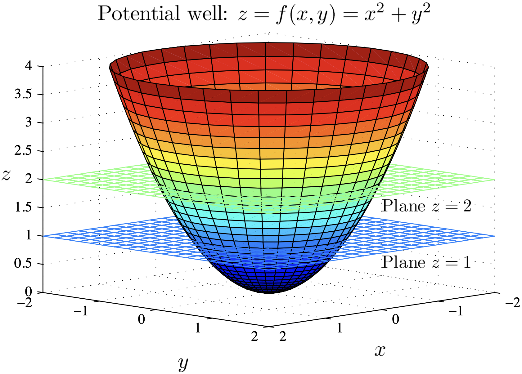
Consider the surface $z=f(x,y)=x^2+y^2$ sliced by horizontal planes $z=0,\,z=1,\,z=2,\dots$
| Plane | Contour | Description |
| $z=0$ | $0 = x^2+ y^2$ | Point $\,(0,0)$ |
| $z=1$ | $1 = x^2+ y^2$ | Circle radius 1, centred at $(0,0)$ |
| $z=2$ | $2 = x^2+ y^2$ | Circle radius $\,\sqrt{2}$ |
| $z=3$ | $3 = x^2+ y^2$ | Circle radius $\,\sqrt{3}$ |
| $z=4$ | $4 = x^2+ y^2$ | Circle radius $\,2$ |
2 Functions of Several Variables
2.3 Contour diagrams
| Plane | Contour | Description |
| $z=0$ | $0 = x^2+ y^2$ | Point $\,(0,0)$ |
| $z=1$ | $1 = x^2+ y^2$ | Circle radius 1, centred at $(0,0)$ |
| $z=2$ | $2 = x^2+ y^2$ | Circle radius $\,\sqrt{2}$ |
| $z=3$ | $3 = x^2+ y^2$ | Circle radius $\,\sqrt{3}$ |
| $z=4$ | $4 = x^2+ y^2$ | Circle radius $\,2$ |
Note that as the radius increases, the contours are more closely spaced.
2 Functions of Several Variables
2.3 Contour diagrams
Note that as the radius increases, the contours are more closely spaced.
2 Functions of Several Variables
2.3 Contour diagrams
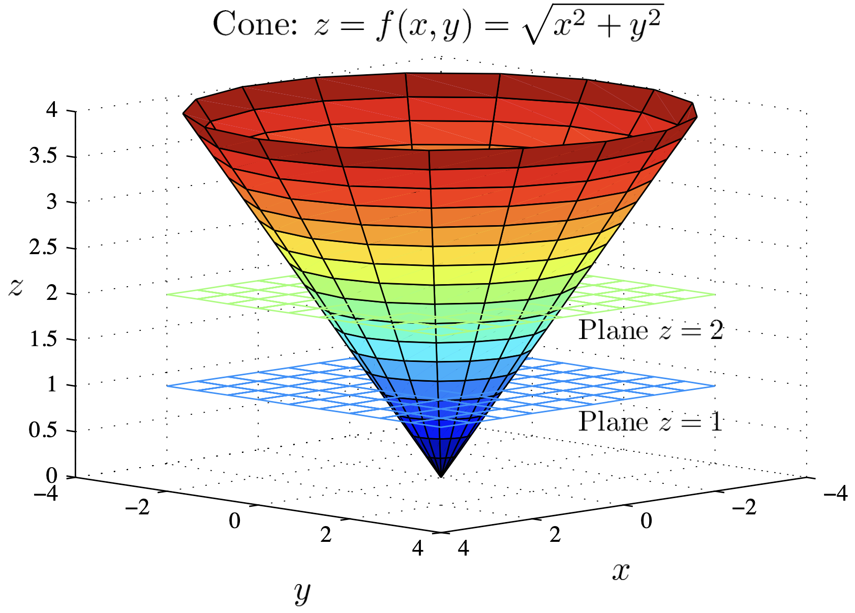
Example: Draw a contour diagram of $f$ given by
$f(x,y)=\sqrt{x^2+y^2}.$
In Matlab, the command is
ezcontour('sqrt(x^2+y^2)', [-10, 10, -10, 10]);
If horizontal planes are equally spaced, say $z=0,$ $\,c,$ $\,2c,$ $\,3c,\dots,$ it is not hard to visualise the surface from its contour diagram. Spread-out contours mean the surface is quite flat and closely spaced ones imply a steep climb.
2 Functions of Several Variables
2.3 Contour diagrams
Example: Draw a contour diagram of $f$ given by $f(x,y)=\sqrt{x^2+y^2}.$
2 Functions of Several Variables
2.3 Contour diagrams
2 Functions of Several Variables
2.3 Contour diagrams
|
|
|
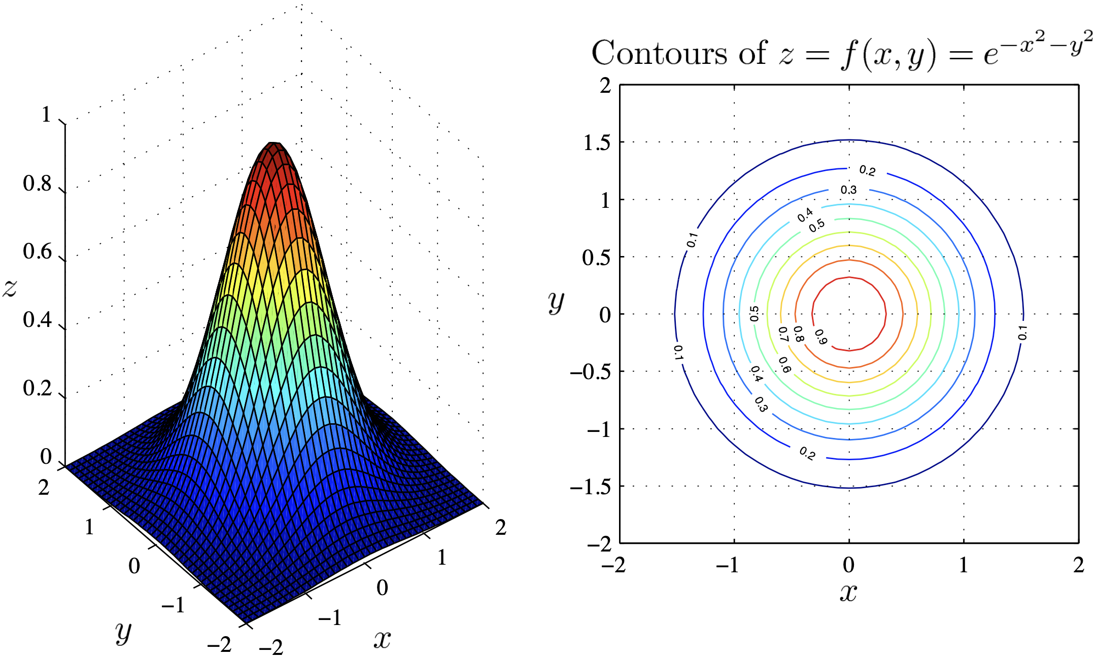
Note that the contours of the last two functions were all circles.
Such surfaces have circular symmetry. When $x$ and $y$ only appear as $x^2+y^2$ in the definition of $f,$ then the graph of $f$ has circular symmetry about the $z$ axis. The height $z$ depends only on the radial distance $r=\sqrt{x^2+y^2}.$
2 Functions of Several Variables
2.3 Contour diagrams
Example: $\,z=f(x,y)=e^{-x^2-y^2}$ $=e^{-\left(x^2+y^2\right)}.$
2 Functions of Several Variables
2.3 Contour diagrams
Example: Draw a contour diagram for $\,z=f(x,y)=x^2+4y^2-2x+1.$
Complete the square: $\,z = \left(x-1\right)^2 -1 + 4y^2+1$
$z = \left(x-1\right)^2 + 4 y^2$
$z \lt 0\, \Ra \,$ no solution.
$z = 0\, \Ra \, x=1, y = 0.$
$z \gt 0\, \Ra \, \ds \frac{\left(x-1\right)^2}{\left(\sqrt{z}\right)^2}+ \frac{y^2}{\left(\frac{\sqrt{z}}{2}\right)^2} = 1 $
2 Functions of Several Variables
2.3 Contour diagrams
Example: Draw a contour diagram for $\,z=f(x,y)=x^2+4y^2-2x+1.$
$z \gt 0\, \Ra \, \ds \frac{\left(x-1\right)^2}{\left(\sqrt{z}\right)^2}+ \frac{y^2}{\left(\frac{\sqrt{z}}{2}\right)^2} = 1 $
| Plane | Contour | Description |
| $z=1$ | $\ds\frac{\left(x-1\right)^2}{\left(\sqrt{1}\right)^2}+ \frac{y^2}{\left(\frac{\sqrt{1}}{2}\right)^2} = 1$ | $a=1,\, b = \dfrac{1}{2}$ |
| $z=2$ | $\ds\frac{\left(x-1\right)^2}{\left(\sqrt{2}\right)^2}+ \frac{y^2}{\left(\frac{\sqrt{2}}{2}\right)^2} = 1$ | $a=\sqrt{2},\, b = \dfrac{\sqrt{2}}{2}$ |
| $z=3$ | $\ds\frac{\left(x-1\right)^2}{\left(\sqrt{3}\right)^2}+ \frac{y^2}{\left(\frac{\sqrt{3}}{2}\right)^2} = 1$ | $a=\sqrt{3},\, b = \dfrac{\sqrt{3}}{2}$ |
2 Functions of Several Variables
2.3 Contour diagrams
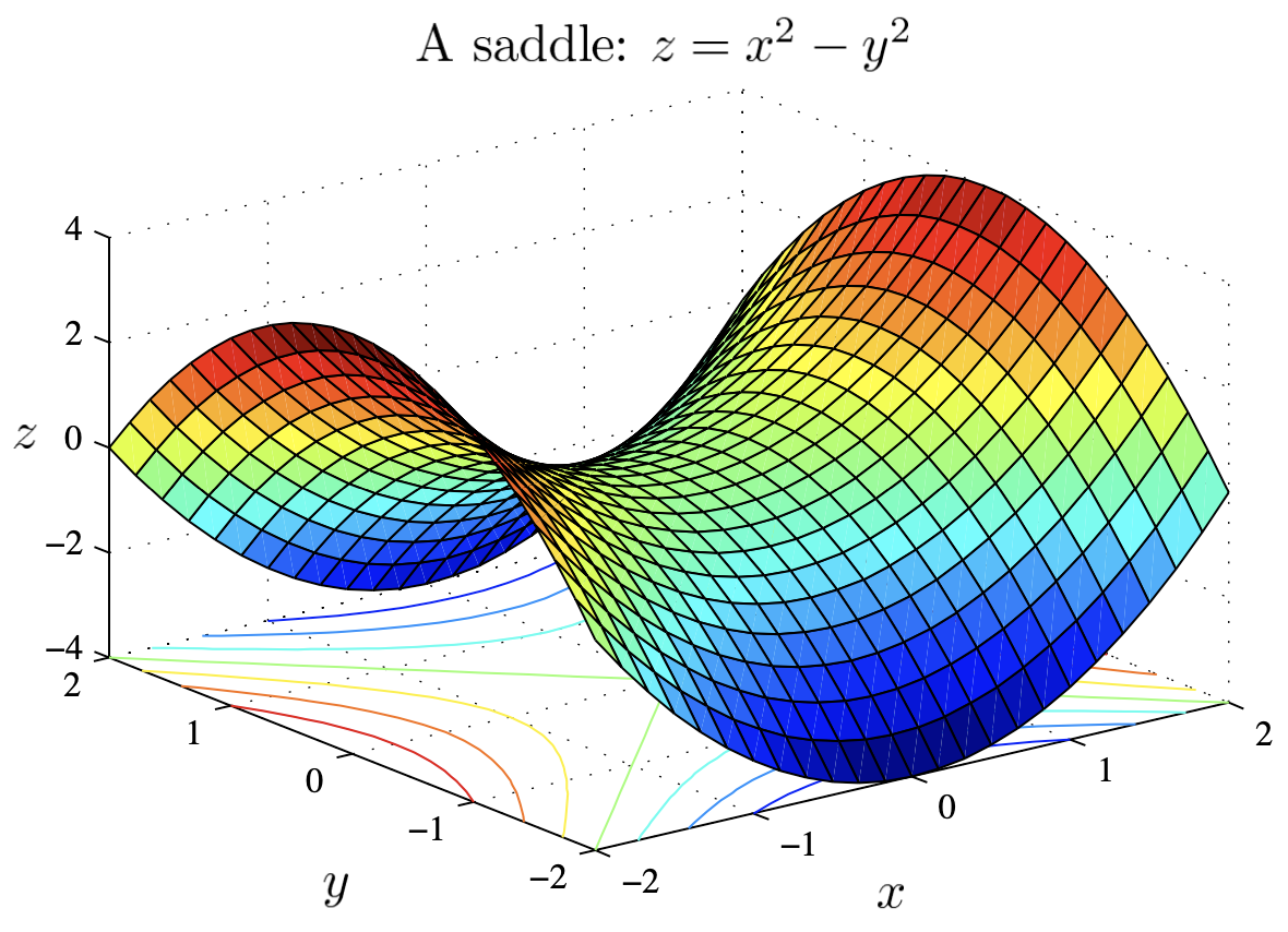
Example: A saddle $z=x^2-y^2$ has hyperbolic contours.
| Plane | Contour |
| $z=0$ |
$\ds 0 = x^2- y^2$
$\ds \, \Ra y^2= x^2$
$\ds \, \Ra y= \pm x$
$\qquad $ $\qquad $ |
| $z=1$ |
$\ds\frac{x^2}{\left(1\right)^2}-
\frac{y^2}{\left(1\right)^2} = 1$
$\qquad $ |
| $z=2$ |
$\ds x^2-y^2 =2$
$\ds\, \Ra \frac{x^2}{\left(\sqrt{2}\right)^2}-
\frac{y^2}{\left(\sqrt{2}\right)^2} = 1$
$\qquad $ |
2 Functions of Several Variables
2.3 Contour diagrams
Example: A saddle $z=x^2-y^2$ has hyperbolic contours.
| Plane | Contour |
| $z=-1$ |
$\ds -1 = x^2- y^2$
$\ds \, \Ra y^2 -x^2=1$
$\qquad $ $\qquad $ $\qquad $ $\qquad $ |
| $z=-2$ |
$\ds x^2-y^2=-2$
$\ds\, \Ra \frac{y^2}{\left(\sqrt{2}\right)^2}-
\frac{x^2}{\left(\sqrt{2}\right)^2}=1$
$\qquad $ $\qquad $ $\qquad $ |
2 Functions of Several Variables
2.3 Contour diagrams
Example: Sketch the contour diagram for $\,z=f(x,y)=9x^2-4y^2+2$ with contours at $\,z=-2,\,2,\,6\,$ and $10.$
$z = -2$ $\, \Ra 9x^2-4y^2+2=-2$
$\, \Ra 9x^2-4y^2=-4$ $\, \ds \Ra \frac{y^2}{1^2}-\frac{x^2}{\left(\frac{2}{3}\right)^2}=1$
Hyperbola: centred at $\,(0,0)\,$ with $a= 2/3, b = 1.$
$\ds \qquad y = \pm \frac{b}{a}x$ $ \ds = \pm \frac{3}{2}x$
2 Functions of Several Variables
2.3 Contour diagrams
Example: Sketch a contour diagram for $\,z=f(x,\,y)=x^2\,$ and use this to sketch the graph of $f.$
$z = 0$ $\, \Ra x^2 = 0$ $\, \Ra x = 0$
$z = 1$ $\, \Ra x^2 = 1$ $\, \Ra x = \pm 1$
$z = 2$ $\, \Ra x^2 = 2$ $\, \Ra x = \pm \sqrt{2}$
2 Functions of Several Variables
2.3 Contour diagrams
Example: Sketch a contour diagram for $\,z=f(x,y)=x-y^2.$
$z = -1$ $\, \Ra x = -1 + y^2$
$z = 0$ $\, \Ra x = y^2$
$z = 1$ $\, \Ra x = 1+ y^2$
$z = 2$ $\, \Ra x = 2 + y^2$
2 Functions of Several Variables
2.3 Contour diagrams
Example: Sketch contour diagrams of
$\,z=f(x,y)=x\;\;$ and $\;\;z=g(x,y)=x+y.$
|
$z = 1$ $\, \Ra x = 1$ $z = 2$ $\, \Ra x = 2$ |
$z = 0$ $\, \Ra y = -x$ $z = 1$ $\, \Ra y = 1-x$ $z = c$ $\, \Ra y = c-x$ |
2 Functions of Several Variables
2.3.1 Main points
-
You should be able to plot contour diagrams in Matlab using the
ezcontourfunction (and its variants). - You should be able to recognise circular symmetry in an equation.
- You should be able to match contour diagrams with functions.
- You should be able to sketch simple contour diagrams.
2 Functions of Several Variables
2.4 Cross-sections of a Surface
A cross-section is the intersection of a surface with a vertical plane such as $y=C,$ see also Stewart Section 12.6.
2 Functions of Several Variables
2.4 Cross-sections of a Surface
A cross-section is the intersection of a surface with a vertical plane such as $y=C$, see also Stewart Section 12.6.
Example:
The height $z$ of a vibrating guitar string can be expressed as a function of horizontal distance $x,$ and time $t$
$z=f(x,t)=A\sin( \pi x) \cos (2 \pi t) \,\, \text{where $\,\, 0 \lt x\lt 1$}.$
$z=f(x,t)=A\sin( \pi x) \cos (2 \pi t) \,\, \text{where $\,\, 0 \lt x\lt 1$}.$
The snapshots where $t$ is constant are cross-sections of the 'surface'.
2 Functions of Several Variables
2.4 Cross-sections of a Surface
Varying time we get
$\quad\qquad t=0:$ $\, \quad z =A\sin (\pi x)$
$\quad\qquad t=\dfrac{1}{8}:$ $ \quad z \ds =\frac{1}{2}\sqrt{2}A\sin (\pi x)$
$\quad\qquad t=\dfrac{1}{4}:$ $ \quad z \ds =0$
$\quad\qquad t=\dfrac{3}{8}:$ $ \quad z \ds =-\frac{1}{2}\sqrt{2}A\sin (\pi x)$
$\quad\qquad t=\dfrac{1}{2}:$ $ \quad z \ds =-A\sin (\pi x)$
These represent sine curves, with amplitudes between $0$ and $A.$
2 Functions of Several Variables
2.4 Cross-sections of a Surface
$\quad\qquad t=0:$ $\, \quad z =A\sin (\pi x)$
$\quad\qquad t=\dfrac{1}{8}:$ $ \quad z \ds =\frac{1}{2}\sqrt{2}A\sin (\pi x)$
$\quad\qquad t=\dfrac{1}{4}:$ $ \quad z \ds =0$
$\quad\qquad t=\dfrac{3}{8}:$ $ \quad z \ds =-\frac{1}{2}\sqrt{2}A\sin (\pi x)$
$\quad\qquad t=\dfrac{1}{2}:$ $ \quad z \ds =-A\sin (\pi x)$
These represent sine curves, with amplitudes between $0$ and $A.$
We can also consider the cross-sections in $x.$ For instance $x=\frac{1}{2}$ (at the top of the sine wave), then $z=A\cos(2 \pi t)$ which equals the amplitude of the sine wave.
2 Functions of Several Variables
2.4 Cross-sections of a Surface
Matlab can be used to make a movie of the 2-dimensional surface by plotting cross-sections at different $t$ values in sequence. The sequence of plots can be stored in a vector and played as a movie using the following code:
								x = (0:0.25:1);
								for j = 1:100
								   t = j/25;
								   z = sin(pi * x) * cos(2 * pi * t);
								   plot(x, z); axis([0,1,-1,1]);
								   M(j) = getframe;
								end
Note:
ezplot cannot be used to do this because
Matlab gets confused
about which of $t$, $x$ is a variable and which is a number.
2 Functions of Several Variables
2.4 Cross-sections of a Surface
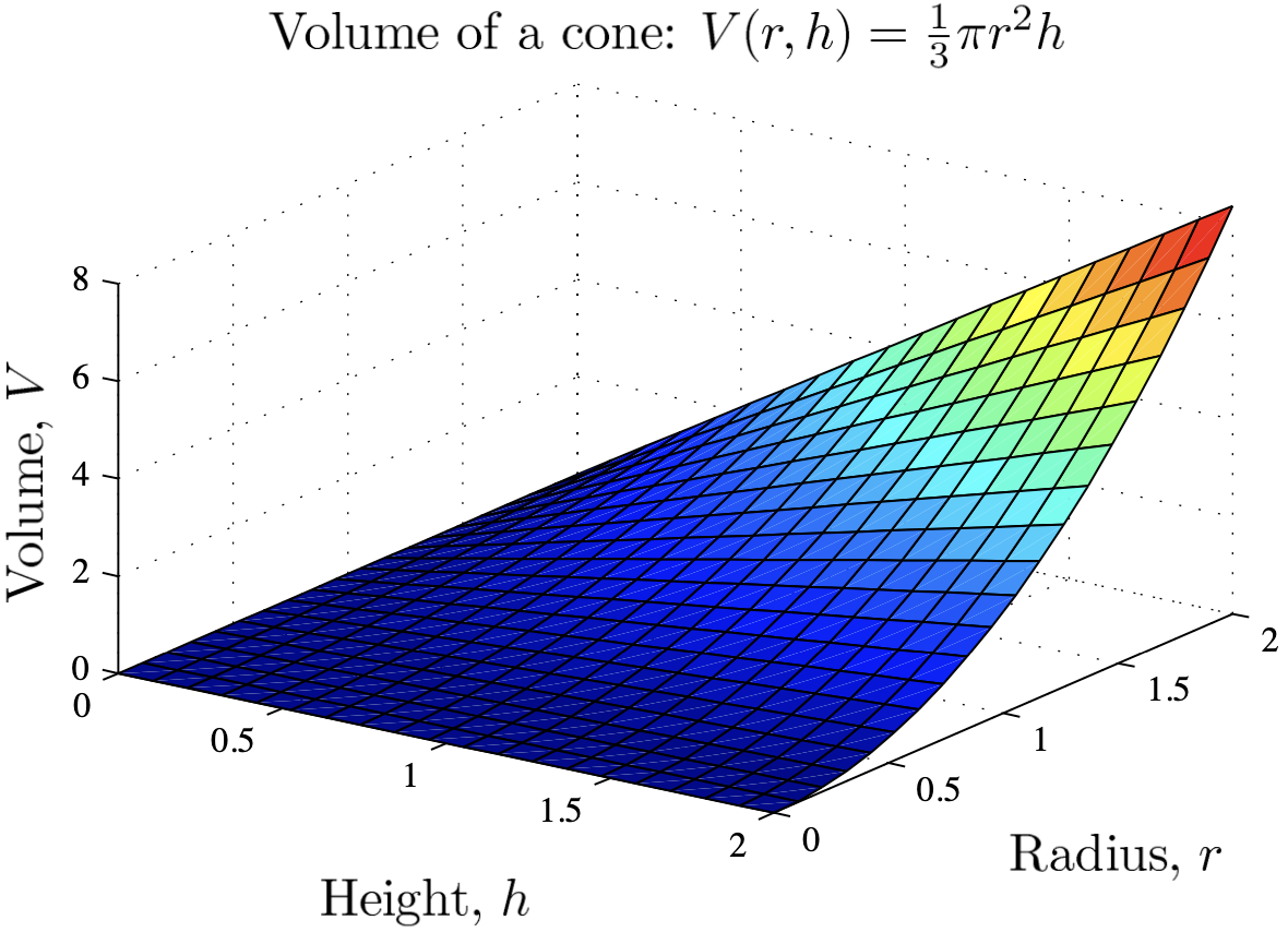
Example: Sketch the cross-sections of the surface $V=\frac13 \pi r^2 h$ (volume of a cone).
2 Functions of Several Variables
2.4 Cross-sections of a Surface
Here is the 3-dimensional picture from Matlab.
2 Functions of Several Variables
2.4 Cross-sections of a Surface
Example: The cross-sections of a saddle $z=x^2-y^2$ are parabolas. For $y=y_0$ they point up: $z=x^2 - (y_0)^2;$ and for $x=x_0$ they point down: $z=-y^2+x_0^2.$
The surface is tricky to draw, unless you are an equestrian.
2 Functions of Several Variables
2.4 Cross-sections of a Surface
Example: The cross-sections of a saddle $z=x^2-y^2$ are parabolas. For $y=y_0$ they point up: $z=x^2 - (y_0)^2;$ and for $x=x_0$ they point down: $z=-y^2+x_0^2.$
The surface is tricky to draw, unless you are an equestrian.
2 Functions of Several Variables
2.4 Cross-sections of a Surface
Here is the 3-dimensional picture from Matlab.
2 Functions of Several Variables
2.4 Cross-sections of a Surface
Example: Use cross-sections to sketch the graph of $z=f(x,y)=x^2$.
2 Functions of Several Variables
2.4.1 Main points
- You should be able to construct cross-sections of multivariate functions.
- Cross sections are 2-dimensional graphs.
- Animation of cross-sections is another way to visualise multivariate functions.
The Gamma function
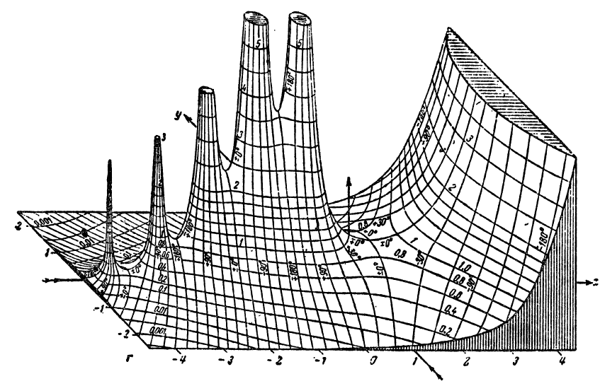
Gamma function by Jahnke and Emde, 1909.
The Gamma function
Source: Analytic landscapes
The big question

Why do I need to learn all these methods to sketch multivariable functions when we already have powerful computational tools to do this job?