Calculus &
Linear Algebra II
Chapter 12
12 Least squares approximation
12.1 Least squares problem - minimising distance to a subspace
A recurring problem in linear algebra, and in its myriad of applications, is the following:
- Given a vector ${\bf v}$ in a real inner product space $V,$ give the best approximation to ${\bf v}$ in a finite-dimensional subspace $U$ of $V.$
This problem is called the "least squares problem".
What do we mean by "best approximation"? It means to find a vector in a subspace of minimal distance to a given vector in the ambient vector space. So the answer to the problem is to
find $\bfu\in U$ such that $d(\bfu,\bfv)$ is as small as possible.
12.1 Least squares problem - minimising distance to a subspace
What do we mean by "best approximation"? It means to find a vector in a subspace of minimal distance to a given vector in the ambient vector space. So the answer to the problem is to
find $\bfu\in U$ such that $d(\bfu,\bfv)$ is as small as possible.
That is, $\mathbf{u}\in U$ that minimises $||\mathbf{v}-\mathbf{u}||.$
Theorem (Best Approximation Theorem). If $U$ is a finite-dimensional subspace of a real inner product space $V,$ and if $\mathbf{v}\in V,$ then $\mathrm{Proj}_U(\bfv)$ is the best approximation to $\mathbf{v}$ from $U$ in the sense that $$||\mathbf{v}-\mathrm{Proj}_U(\bfv)|| \leq ||\mathbf{v}-\mathbf{u}||, ~~\forall \mathbf{u}\in U.$$
12.1 Least squares problem - minimising distance to a subspace
12.1 Least squares problem - minimising distance to a subspace
Theorem (Best Approximation Theorem). If $U$ is a finite-dimensional subspace of a real inner product space $V,$ and if $\mathbf{v}\in V,$ then $\mathrm{Proj}_U(\bfv)$ is the best approximation to $\mathbf{v}$ from $U$ in the sense that $||\mathbf{v}-\mathrm{Proj}_U(\bfv)|| \leq ||\mathbf{v}-\mathbf{u}||, ~~\forall \mathbf{u}\in U.$
Proof: Let $U$ be a finite-dimensional subspace of $V$ and $\v \in V$, $\u\in U$. Then
$ \norm{ \v - \mathrm{Proj}_U(\bfv) }^2 \leq \norm{ \v - \mathrm{Proj}_U(\bfv) }^2+ \norm{ \mathrm{Proj}_U(\bfv) -\u }^2$
$ \norm{ \v - \mathrm{Proj}_U(\bfv) }^2 \leq \underbrace{\norm{ \v - \mathrm{Proj}_U(\bfv) }^2}_{{\Large \in U^{\perp}}}+ \underbrace{\norm{ \mathrm{Proj}_U(\bfv) -\u }^2}_{{\Large \in U}}$
$ \qquad\quad\qquad \leq \norm{ \v - \mathrm{Proj}_U(\bfv) + \mathrm{Proj}_U(\bfv) -\u }^2 $
$ \leq \norm{ \v -\u }^2.\qquad\quad\, $
Therefore $\norm{ \v - \mathrm{Proj}_U(\bfv) } \leq \norm{ \v -\u }$ for all $\u\in U. \qquad \blacksquare$
12.1 Least squares problem - minimising distance to a subspace
From the Best Approximation Theorem, $\u = \mathrm{Proj}_U(\bfv)$ is the best approximation to $\v \in V$ in a finite-dimensional subspace $U$ of $V$.
How to find $\mathrm{Proj}_U(\bfv)$?
Solution 1. Use Gram-Schmidt process to construct an orthonormal basis $\{\bfe_1, \bfe_2,\cdots,\bfe_n\}$ of $U.$ Then $$ \mathrm{Proj}_U(\bfv)= \langle\bfv,\bfe_1\rangle\bfe_1+\ldots+\langle\bfv,\bfe_n\rangle\bfe_n. $$
Solution 2. Let $\gamma=\{\bfu_1, \bfu_2,\cdots,\bfu_n\}$ be a basis of the subspace $U$. Then any $\u \in U$ can be written as $\u = \alpha_1 \u_1+ \alpha_2 \u_2+ \cdots \alpha_n \u_n.$
12.1 Least squares problem - minimising distance to a subspace
Solution 2. Let $\gamma=\{\bfu_1, \bfu_2,\cdots,\bfu_n\}$ be a basis of the subspace $U.$ Then any $\u \in U$ can be written as $\u = \alpha_1 \u_1+ \alpha_2 \u_2+ \cdots \alpha_n \u_n.$
We seek coefficients $\alpha_1,\alpha_2,\dots \alpha_n$ that minimise $||\mathbf{v}-\u||,$ or equivalently, minimise $||\mathbf{v}-\u||^2=||\mathbf{v}-(\alpha_1 \mathbf{u}_1+\alpha_2 \mathbf{u}_2+\dots +\alpha_n \mathbf{u}_n)||^2$ (same outcome, avoid square root).
$||\mathbf{v}-(\alpha_1 \mathbf{u}_1+\alpha_2 \mathbf{u}_2+\dots +\alpha_n \mathbf{u}_n)||^2$
$\;\;=\langle \mathbf{v}-(\alpha_1 \mathbf{u}_1+\alpha_2 \mathbf{u}_2+\dots +\alpha_n \mathbf{u}_n), \mathbf{v}-(\alpha_1 \mathbf{u}_1+\alpha_2 \mathbf{u}_2+\dots +\alpha_n \mathbf{u}_n) \rangle$
$\;\;=\langle \mathbf{v},\mathbf{v} \rangle-2\alpha_1 \langle \mathbf{v},\mathbf{u}_1 \rangle -2\alpha_2 \langle \mathbf{v},\mathbf{u}_2 \rangle -\dots-2\alpha_n \langle \mathbf{v},\mathbf{u}_n \rangle +\sum_{i=1}^n\sum_{j=1}^n\alpha_i\alpha_j \langle \mathbf{u}_i, \mathbf{u}_j \rangle$
$\;\;=E(\alpha_1,\alpha_2,\dots,\alpha_n).$
$E$ is a real valued function and is called the "error".
12.1 Least squares problem - minimising distance to a subspace
From MATH1052/MATH1072: we minimise $E$. Set $\nabla E=\mathbf{0},$ which gives \begin{align*} \frac{\partial E}{\partial \alpha_k}=-2\langle \mathbf{v},\mathbf{u}_k \rangle+2\sum_{l=1}^n \alpha_l \langle\mathbf{u}_k,\mathbf{u}_l \rangle=0. \end{align*}
This is $n$ equations in $n$ unknowns, which may be expressed in matrix form: \begin{align*} \left( \begin{array}{cccc} \langle \mathbf{u}_1,\mathbf{u}_1\rangle ~ & \langle \mathbf{u}_1,\mathbf{u}_2\rangle ~\dots ~ \langle \mathbf{u}_1,\mathbf{u}_n\rangle \\ \langle \mathbf{u}_2,\mathbf{u}_1\rangle ~ & \langle \mathbf{u}_2,\mathbf{u}_2\rangle ~\dots ~ \langle \mathbf{u}_2,\mathbf{u}_n\rangle\\ \vdots&~\vdots & \\ \langle \mathbf{u}_n,\mathbf{u}_1\rangle ~ & \langle \mathbf{u}_n,\mathbf{u}_2\rangle ~\dots ~ \langle \mathbf{u}_n,\mathbf{u}_n\rangle \end{array} \right) \left(\begin{array}{c} \alpha_1\\ \alpha_2\\ \vdots\\ \alpha_n \end{array}\right)&= \left(\begin{array}{c} \langle \mathbf{v},\mathbf{u}_1 \rangle\\ \langle \mathbf{v},\mathbf{u}_2 \rangle \\ \vdots\\ \langle \mathbf{v},\mathbf{u}_n \rangle \end{array}\right). \end{align*}
12.1 Least squares problem - minimising distance to a subspace
This is $n$ equations in $n$ unknowns, which may be expressed in matrix form: \begin{align*} \left(~~~ \begin{array}{cccc} \langle \mathbf{u}_1,\mathbf{u}_1\rangle & \langle \mathbf{u}_1,\mathbf{u}_2\rangle & \dots & \langle \mathbf{u}_1,\mathbf{u}_n\rangle \\ \langle \mathbf{u}_2,\mathbf{u}_1\rangle & \langle \mathbf{u}_2,\mathbf{u}_2\rangle & \dots & \langle \mathbf{u}_2,\mathbf{u}_n\rangle \\ \vdots & & \vdots & & \\ \langle \mathbf{u}_n,\mathbf{u}_1\rangle & \langle \mathbf{u}_n,\mathbf{u}_2\rangle & \dots & \langle \mathbf{u}_n,\mathbf{u}_n\rangle \end{array} \right) \left(\begin{array}{c} \alpha_1\\ \alpha_2\\ \vdots\\ \alpha_n \end{array}\right)&= \left(\begin{array}{c} \langle \mathbf{v},\mathbf{u}_1 \rangle\\ \langle \mathbf{v},\mathbf{u}_2 \rangle \\ \vdots\\ \langle \mathbf{v},\mathbf{u}_n \rangle \end{array}\right). \end{align*}
Solve this system for $\alpha_1, \alpha_2, \ldots,\alpha_n$ to obtain \[ \mathrm{Proj}_U(\bfv) = \alpha_1\u_1+ \alpha_2\u_2+\cdots + \alpha_n\u_n. \]
Note: If $\gamma$ is orthonormal $\implies$ matrix on LHS$\,=I$ (the identity matrix) $\implies$ $\alpha_i=\langle \mathbf{v}, \mathbf{u}_i\rangle,$ which coincides with Solution 1, as expected.
12.2 Inconsistent linear systems
In applications, one is often faced with over-determined linear systems. For example, we may have a bunch of data points that we have reasons to believe should fit on a straight line. But real-life data points rarely match predictions exactly.
The goal in this section is to develop a method for obtaining the best fit or approximation of a specified kind to a given set of data points.
12.2 Inconsistent linear systems
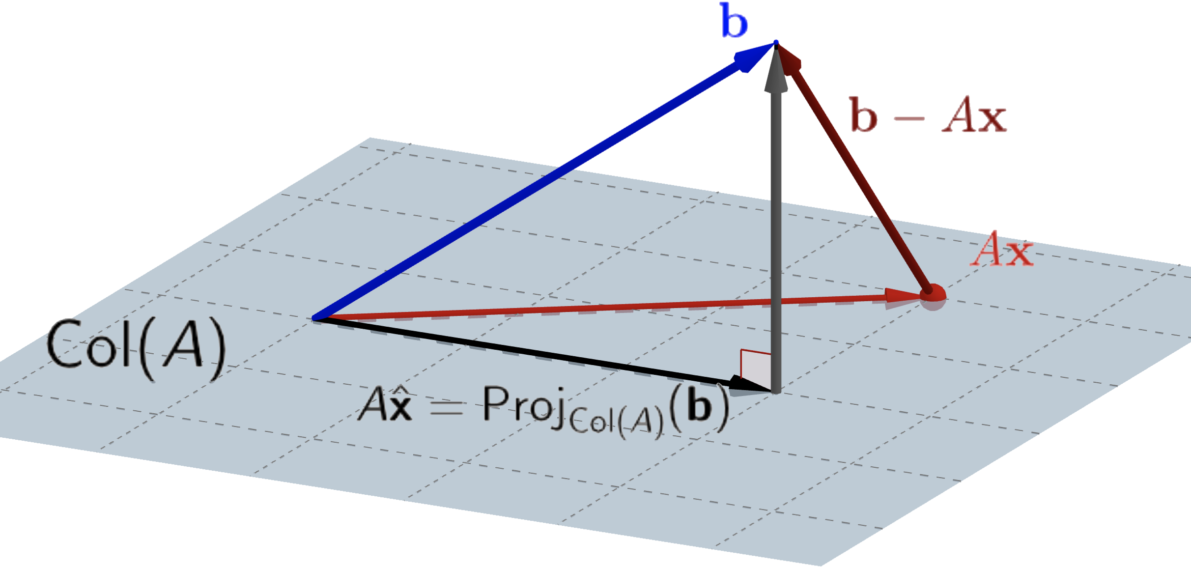
To this end, let $A\in M_{m,n}(\mathbb{R})$ and ${\bf b}\in M_{m,1}(\mathbb{R}).$ For $m>n,$ the linear system described by $A{\bf x}={\bf b}$ is over-determined and does not in general have a solution. However, we may be satisfied if we can find $\hat{\bf x}\in M_{n,1}(\mathbb{R})$ such that $A\hat{\bf x}$ is as 'close' to ${\bf b}$ as possible. That is, we seek to minimise $||{\bf b}-A{\bf x}||$ for given $A$ and ${\bf b}$. For computational reasons, one usually minimises $||{\bf b}-A{\bf x}||^2$ instead.
A solution $\hat{\bf x}$ to this minimisation problem is referred to as a least squares solution.
12.2 Inconsistent linear systems
We seek to minimise $||{\bf b}-A{\bf x}||$ for given $A$ and ${\bf b}$. For computational reasons, one usually minimises $||{\bf b}-A{\bf x}||^2$ instead. A solution $\hat{\bf x}$ to this minimisation problem is referred to as a least squares solution.
12.2 Inconsistent linear systems
To find $\hat{\bf x},$ let us recall the column space of the matrix $A$. Let ${\bf a}_1,\ldots,{\bf a}_n\in M_{m,1}(\mathbb{R})$ be the columns of $A$, i.e., $A = \left({\bf a}_1 ~|~ {\bf a}_2 ~|~\cdots ~|~{\bf a}_n\right)$, then $$\mathrm{Col}(A)=\mathrm{span}(\{{\bf a}_1,\ldots,{\bf a}_n\}).$$
Let ${\bf x}\in M_{n,1}(\mathbb{R})$ then we have \begin{align*} A{\bf x}& = A \begin{pmatrix} x_1\\ x_2\\ \vdots\\ x_n\end{pmatrix} = x_1{\bf a}_1+x_2{\bf a}_2+\cdots + x_n{\bf a}_n,\quad x_k\in \R. \end{align*} So $A{\bf x}$ is a linear combination of the columns of $A,$ i.e., a vector of the form $A{\bf x}$ is always a vector in $\mathrm{Col}(A).$
12.2 Inconsistent linear systems
Let ${\bf x}\in M_{n,1}(\mathbb{R})$ then we have \begin{align*} A{\bf x}& = A \begin{pmatrix} x_1\\ x_2\\ \vdots\\ x_n\end{pmatrix} = x_1{\bf a}_1+x_2{\bf a}_2+\cdots + x_n{\bf a}_n,\quad x_k\in \R. \end{align*} So $A{\bf x}$ is a linear combination of the columns of $A,$ i.e., a vector of the form $A{\bf x}$ is always a vector in $\mathrm{Col}(A).$
It follows that $A\hat{\bf x}\in\mathrm{Col}(A)$. We are thus in the situation described in Section 12.1.
12.2 Inconsistent linear systems
It follows that $A\hat{\bf x}\in\mathrm{Col}(A).$ We are thus in the situation described in Section 12.1.
For a finite-dimensional subspace $U\subset V $ and $\v\in V$ and
$\u \in U,$
$\u = \mathrm{Proj}_{U}({\bf v})$ minimizes $\norm{\v-\u}^2.$
Hence $U = \mathrm{Col}(A)$ and $\v= \mathbf b$
with all vectors in $U$ of the form $A \mathbf x$.
Then $$\mathrm{Proj}_{\mathrm{Col}(A)}({\bf b})$$ is a vector in $\mathrm{Col}(A)$.
12.2 Inconsistent linear systems
It follows that $A\hat{\bf x}\in\mathrm{Col}(A).$ We are thus in the situation described in Section 12.1.
12.2 Inconsistent linear systems
Consequently, we know that $$ A\hat{\bf x}=\mathrm{Proj}_{\mathrm{Col}(A)}({\bf b}). $$ But we are still faced with the task of disentangling $\hat{\bf x}$. Note that, although $A\hat{\bf x}=\mathrm{Proj}_{\mathrm{Col}(A)}({\bf b})$ is uniquely given in terms of $A$ and ${\bf b},$ its solution $\hat{\bf x}$ need not be.
Solution 3. For the current special application, i.e. least squares solutions of linear systems, we have a more direct (and simpler) method. In the following we describe this method and give some examples.
12.3 $\mathrm{Col}(A)^\bot=N\left(A^T\right)$
The orthogonal complement of the column space of $A$ is the null space of $A^T$.
Note: Recall that $\left(A\v\right)\pd \u = \left(A\v\right)^T \u = \v^T A^T \u = \v \pd \left(A^T\u\right)$. $\quad(\star)$
Proof: $\subseteq$ - Let $\u\in \mathrm{Col}(A)^{\perp},$ then for $\v \in \R^n$
$ 0 = \left(A \v\right)\pd \u $ $ = \left(A \v\right)^T \u $ $ = \v^TA^T \u $ $ = \v \pd \left(A^T \u\right) $
Set $\v = A^T\u$, then $0 = \left(A^T \u\right) \pd \left(A^T \u\right) $ $\; \Ra\; A^T\u = \mathbf 0 $
$\; \Ra \;\u \in N\left(A^T\right) $ $\; \Ra \; \mathrm{Col}(A)^{\perp} \subseteq N\left(A^T\right) .$
12.3 $\mathrm{Col}(A)^\bot=N\left(A^T\right)$
The orthogonal complement of the column space of $A$ is the null space of $A^T$.
Note: Recall that $\left(A\v\right)\pd \u = \left(A\v\right)^T \u = \v^T A^T \u = \v \pd \left(A^T\u\right)$. $\quad(\star)$
$\supseteq$ - Let $\u\in N\left(A^T\right),$ then for $A^T \u = \mathbf 0$. Thus for all $\v \in \R^n$ we have
$ 0 =\v \pd \mathbf 0 $ $ = \v \pd \left(A^T \u\right) $ $ = \v^TA^T \u $ $ = \left(A\v\right)^T \u $ $ = \left(A\v\right) \pd \u $
So $\u$ is perpendicular to all vectors of the form $A \v\in \mathrm{Col}(A)$
$ \; \Ra \;\u \in \mathrm{Col}(A)^{\perp} $ $ \; \Ra \;\mathrm{Col}(A)^{\perp} \supseteq N\left(A^T\right). $ $ \quad \blacksquare $
12.4 Solving for $\hat{\bf x}$
Recall from Section 11.4 that $\bfv-\mathrm{Proj}_U(\bfv)=\mathrm{Proj}_{U^\bot}(\bfv)\in U^\bot$ for any finite-dimensional subspace $U$ of $V$ and $\bfv\in V,$ Since $A\hat{\bf x}=\mathrm{Proj}_{\mathrm{Col}(A)}({\bf b}),$ we thus have $$ {\bf b}-A\hat{\bf x}\in\mathrm{Col}(A)^\bot. $$
12.4 Solving for $\hat{\bf x}$
Recall from Section 11.4 that $\bfv-\mathrm{Proj}_U(\bfv)=\mathrm{Proj}_{U^\bot}(\bfv)\in U^\bot$ for any finite-dimensional subspace $U$ of $V$ and $\bfv\in V.$ Since $A\hat{\bf x}=\mathrm{Proj}_{\mathrm{Col}(A)}({\bf b}),$ we thus have $$ {\bf b}-A\hat{\bf x}\in\mathrm{Col}(A)^\bot. $$
Because $\mathrm{Col}(A)^\bot=N\left(A^T\right),$ it follows that $A^T({\bf b}-A\hat{\bf x})={\bf 0},$ so $$ A^T\!A\hat{\bf x}=A^T{\bf b}. $$
12.4 Solving for $\hat{\bf x}$
Since $A\in M_{m,n}(\mathbb{R})\; \Rightarrow\; A^T\!A\in M_{n,n}(\mathbb{R}),$ the equation $A^T\!A\hat{\bf x}=A^T{\bf b}$ can always be solved for $\hat{\bf x},$ for example by Gaussian elimination. However, the solution need not be unique. Indeed, the solution is unique if and only if $A^T\!A$ is invertible, in which case $$ \hat{{\bf x}}=\left(A^T\!A\right)^{-1}A^T{\bf b}. $$ A key to determining whether $A^T\!A$ is invertible is the following result:
$\{{\bf a}_1,\ldots,{\bf a}_n\}$ is linearly independent $\;\Longleftrightarrow\;$ $A^TA$ is invertible.
12.4 Solving for $\hat{\bf x}$
$\{{\bf a}_1,\ldots,{\bf a}_n\}$ is linearly independent $\;\Longleftrightarrow\;$ $A^TA$ is invertible.
To prove this result, first we will prove the following
Lemma: $N(A) = N\left(A^TA\right).$
Proof: "$\subseteq$" - For $\v \in N(A) $ $\;\Ra\; A\v = \mathbf 0$ $\;\Ra\; A^T\v = \mathbf 0$ $\;\Ra\; \v \in N\left(A^TA\right).$
"$\supseteq$" - For $\v \in N\left(A^TA\right) $ $\;\Ra\; A^TA\v = \mathbf 0$
$\;\Ra\; \mathbf 0 = \v \pd \mathbf 0$ $= \v \pd \left(A^TA \v\right)$ $= \v^T A^T A \v$ $= \left(A\v \right)^T A \v$ $= \left(A\v \right)\pd \left(A\v \right)$
$\;\Ra\; A\v = \mathbf 0$ $\;\Ra\; \v = \mathbf 0$ $\;\Ra\; \v \in N(A).$ $\quad \blacksquare$
12.4 Solving for $\hat{\bf x}$
$\{{\bf a}_1,\ldots,{\bf a}_n\}$ is linearly independent $\;\Longleftrightarrow\;$ $A^TA$ is invertible.
Proof: The set $\left\{{\bf a}_1,\ldots,{\bf a}_n\right\}$ is linearly independent if and only if
$N(A) = \{\mathbf 0\}$ $\;\iff \; N\left(A^TA\right) = \{\mathbf 0\}\;$ by previous Lemma
$\;\iff \;$ $A^TA$ is invertible. $\quad \blacksquare$
12.4 Solving for $\hat{\bf x}$
🤔 But how does that help?
Well, recall that $m>n$ so that $A$ may be describing an
over-determined linear system.
In fact, in case the linear system encodes experimental or
empirical data, $m$ is likely to be much larger than $n$.
The columns of $A$ are then very likely to be linearly
independent, and $A^TA$ would indeed be invertible.
12.5 Fitting a curve to data
Experiments yield data (assume $x_i$ distinct and exact) $$ (x_1, y_1),\;(x_2,y_2),\;\cdots, \;(x_n, y_n) $$ which include measurement error. Theory may predict polynomial relation between $x$ and $y$. But experimental data points rarely match theoretical predictions exactly.
We seek a least squares polynomial function of best fit (e.g. least squares line of best fit or regression line).
12.5 Fitting a curve to data
We seek a least squares polynomial function of best fit (e.g. least squares line of best fit or regression line).
12.5 Fitting a curve to data
Example: Quadratic fit. Suppose some physical system is modeled by a quadratic function $p(t).$ Data in the form $(t,p(t))$ have been recorded as $$ (1,5),\ (2,2),\ (4,7),\ (5,10). $$ Find the least squares approximation for $p(t)$.
12.5 Fitting a curve to data
Example: Quadratic fit. Suppose some physical system is modeled by a quadratic function $p(t).$ Data in the form $(t,p(t))$ have been recorded as $$ (1,5),\ (2,2),\ (4,7),\ (5,10). $$ Find the least squares approximation for $p(t).$
Consider the quadratic function $p(t) = a_0 + a_1 t + a_2 t^2$. To find the least squares approximation we need to solve the linear system:
\[ \left\{ \begin{array}{ccccccc} a_0& +& a_1 (1)& + & a_2 (1)^2 & = & 5 \\ a_0& + &a_1 (2) &+ &a_2 (2)^2 & = & 2 \\ a_0 &+& a_1 (4) &+ &a_2 (4)^2 & = & 7 \\ a_0 &+& a_1 (5)& +& a_2 (5)^2 & = & 10 \\ \end{array} \right. \]
\[ \left\{ \begin{array}{ccrcrcc} a_0& +& a_1 & + & a_2 & = & 5 \\ a_0& + & 2a_1 &+ & 4a_2 & = & 2 \\ a_0 &+& 4a_1 &+ & 16a_2 & = & 7 \\ a_0 &+& 5a_1 & +& 25a_2 & = & 10 \\ \end{array} \right. \]
\[ \left( \begin{array}{ccc} 1 & 1 & 1 \\ 1 & 2 & 4 \\ 1 & 4 & 16 \\ 1 & 5 & 25 \\ \end{array} \right) \left( \begin{array}{c} a_0 \\ a_1 \\ a_2 \\ \end{array} \right) = \left( \begin{array}{c} 5 \\ 2 \\ 7 \\ 10 \\ \end{array} \right) \]
\[ \underbrace{\left( \begin{array}{ccc} 1 & 1 & 1 \\ 1 & 2 & 4 \\ 1 & 4 & 16 \\ 1 & 5 & 25 \\ \end{array} \right)}_{{\Large A}} \underbrace{\left( \begin{array}{c} a_0 \\ a_1 \\ a_2 \\ \end{array} \right)}_{{\Large \mathbf x}} = \underbrace{\left( \begin{array}{c} 5 \\ 2 \\ 7 \\ 10 \\ \end{array} \right)}_{{\Large \mathbf b}} \]
12.5 Fitting a curve to data
Example: Quadratic fit. Suppose some physical system is modeled by a quadratic function $p(t).$ Data in the form $(t,p(t))$ have been recorded as $$ (1,5),\ (2,2),\ (4,7),\ (5,10). $$ Find the least squares approximation for $p(t).$
\[ \underbrace{\left( \begin{array}{ccc} 1 & 1 & 1 \\ 1 & 2 & 4 \\ 1 & 4 & 16 \\ 1 & 5 & 25 \\ \end{array} \right)}_{A} \underbrace{\left( \begin{array}{c} a_0 \\ a_1 \\ a_2 \\ \end{array} \right)}_{\mathbf x} = \underbrace{\left( \begin{array}{c} 5 \\ 2 \\ 7 \\ 10 \\ \end{array} \right)}_{\mathbf b} \]
So we have $A\mathbf x = \mathbf b$. This is an over-determined and inconsistent system but the columns of $A$ are linearly independent. Then $A^TA$ is invertible.
12.5 Fitting a curve to data
Example: Quadratic fit. Suppose some physical system is modeled by a quadratic function $p(t).$ Data in the form $(t,p(t))$ have been recorded as $$ (1,5),\ (2,2),\ (4,7),\ (5,10). $$ Find the least squares approximation for $p(t).$
\[\Ra\;\; \underbrace{\left( \begin{array}{ccc} 1 & 1 & 1 & 1\\ 1 & 2 & 4 & 5\\ 1 & 4 & 16 & 25 \end{array} \right)}_{A^T} \underbrace{\left( \begin{array}{ccc} 1 & 1 & 1 \\ 1 & 2 & 4 \\ 1 & 4 & 16 \\ 1 & 5 & 25 \\ \end{array} \right)}_{A} \underbrace{\left( \begin{array}{c} a_0 \\ a_1 \\ a_2 \\ \end{array} \right)}_{\mathbf x} = \underbrace{\left( \begin{array}{ccc} 1 & 1 & 1 & 1\\ 1 & 2 & 4 & 5\\ 1 & 4 & 16 & 25 \end{array} \right)}_{A^T} \underbrace{\left( \begin{array}{c} 5 \\ 2 \\ 7 \\ 10 \\ \end{array} \right)}_{\mathbf b} \]
Since $\,A^TA\,$ is invertible, then the least squares approximation is
$\ds \hat{\mathbf x} = \left(A^T A\right)^{-1}A^T \mathbf b$ $= \left( \begin{array}{r} 8 \\ -\dfrac{9}{2} \\ 1 \\ \end{array} \right) $ $\;\,\Ra \;\, p(t) = 8 - \dfrac{9}{2}t+ t^2. $
Quadratic fit
Data: $(1,5),\ (2,2),\ (4,7),\ (5,10).$