Strange Attractors
Interactive 3D simulations
By Juan Carlos Ponce Campuzano, 15/August/2018
Introduction
In dynamical systems, a 'Strange Attractor' is a type of attractor (a region or shape to which points are 'pulled' as the result of a certain process) that arises in certain non-linear systems and is characterized by its fractal structure. Unlike regular attractors, which maybe points, close loops, or more complex but still regular shapes, a strange attractor, is highly sensitive to small changes in the initial conditions, leading to chaotic behaivor within the system (Schuster 1989, pp. 105-106; Strogatz 2018, chapter 9). The name was instroduced in the early 1970s by David Ruelle and Floris Takens in a paper in which they proposed that fluid turbulence is an example of what we now call chaos (Lorenz 1993, p. 48; Ruelle & Takens 1971).
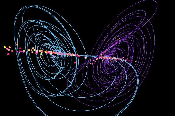
The most famous strange attractor is undoubtedly the Lorenz attractor - a three dimensional object whose body plan resembles a butterfly or a mask. The Lorenz attractor, named for its discoverer Edward N. Lorenz, arose from a mathematical model of the atmosphere (Lorenz 1963).
Imagine a rectangular slice of air heated from below and cooled from above by edges kept at constant temperatures. This is our atmosphere in its simplest description. The bottom is heated by the earth and the top is cooled by the void of outer space. Within this slice, warm air rises and cool air sinks. The state of the atmosphere in this model can be described by three time-evolving variables
- x = the convective flow
- y = the horizontal temperature distribution
- z = the vertical temperature distribution
- $\sigma$ [sigma] = the ratio of viscosity to thermal conductivity
- $\rho$ [rho] = the temperature difference between the top and bottom of the slice
- $\beta$ [beta] = the width to height ratio of the slice
If you want to know how to plot the Lorenz attractor with GeoGebra, check the tutorial below:
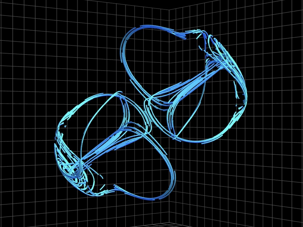
The Lorenz attractor was the first strange attractor, but there are many systems of equations that give rise to strange attractors. In the next section you will find simulations of strange attractors with particles moving based on the given system of ordinary differential equations, including one (or two) solution curve(s). Change the parameters to observe the behaviour of the particles and the solution curve(s). To access the simulation just click on the image.
Interactive simulations
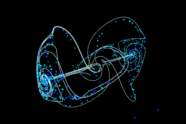
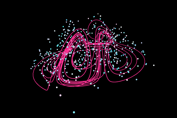
Thomas
Parameter:
$b=0.208186$
System:
$\left\{ \begin{eqnarray*} \frac{dx}{dt}&=&\sin y -bx\\ \frac{dy}{dt}&=&\sin z -by\\ \frac{dz}{dt}&=&\sin x-bz \end{eqnarray*}\right. $
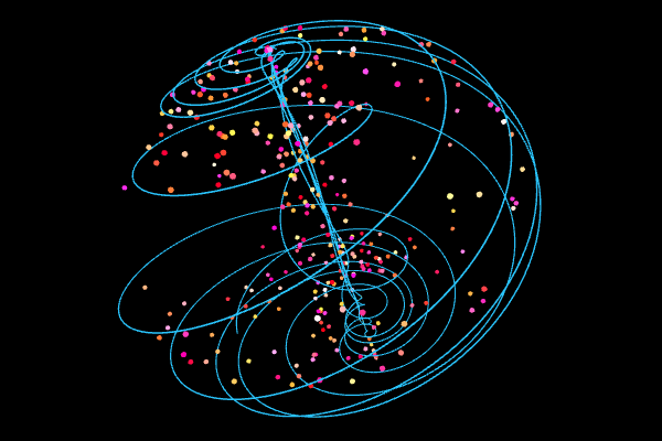
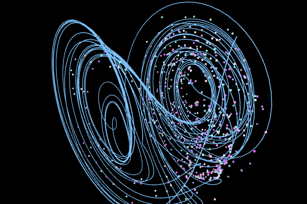
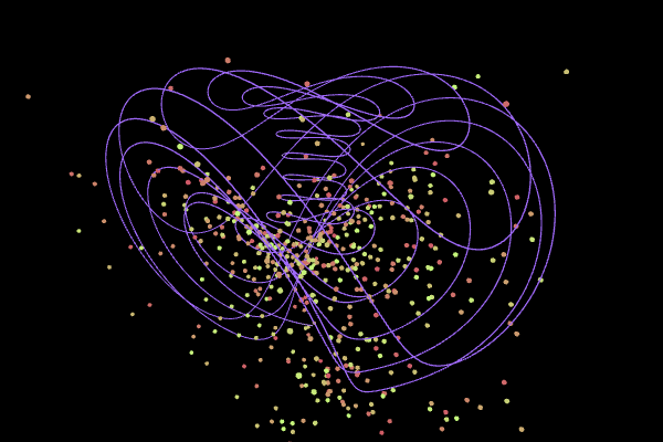
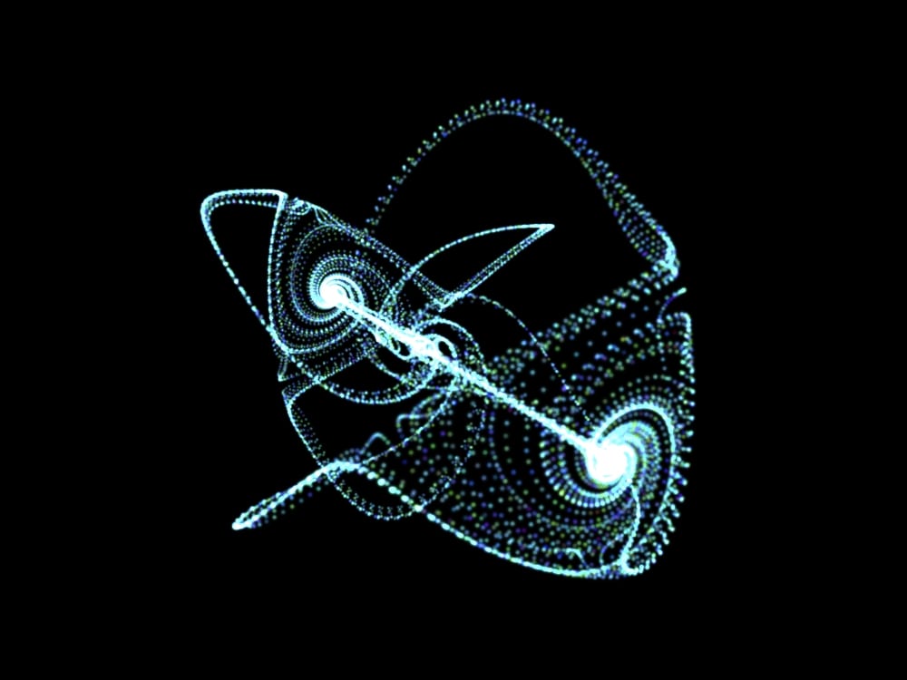
Langford (a.k.a Aizawa)
Parameters:
$a = 0.95,$ $b = 0.7,$ $c = 0.6,$
$d = 3.5,$ $e = 0.25,$ $f = 0.1$
System:
$\left\{ \begin{eqnarray*} \frac{dx}{dt}&=&(z - b) x - d y\\ \frac{dy}{dt}&=& d x + (z - b) y\\ \frac{dz}{dt}&=&c + a z - \frac{z^3}{3} \\& &\;\;\;-(x^2+y^2)(1+e z)+f z x^3 \end{eqnarray*}\right. $
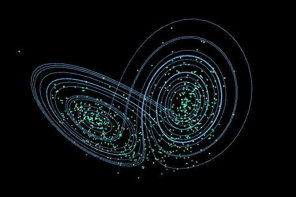
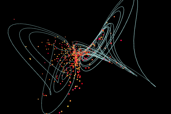
Lorenz
Parameters:
$\sigma = 10,$ $\rho = 28,$ $\beta = 8/3$
System:
$\left\{ \begin{eqnarray*} \frac{dx}{dt}&=&\sigma (-x + y)\\ \frac{dy}{dt}&=& -x z + \rho x - y \\ \frac{dz}{dt}&=& x y - \beta z \end{eqnarray*}\right. $
Dadras
Parameters:
$a = 3,$ $b = 2.7,$ $c = 1.7,$
$d = 2,$ $e = 9$
System:
$\left\{ \begin{eqnarray*} \frac{dx}{dt}&=& y - a x +b y z\\ \frac{dy}{dt}&=& c y - x z +z\\ \frac{dz}{dt}&=& d x y - e z \end{eqnarray*}\right. $
Chen
Parameters:
$\alpha = 5$, $\beta = -10$, $\delta = -0.38$
System:
$\left\{ \begin{eqnarray*} \frac{dx}{dt}&=&\alpha x- y z\\ \frac{dy}{dt}&=&\beta y + x z \\ \frac{dz}{dt}&=&\delta z + x y/3 \end{eqnarray*}\right. $
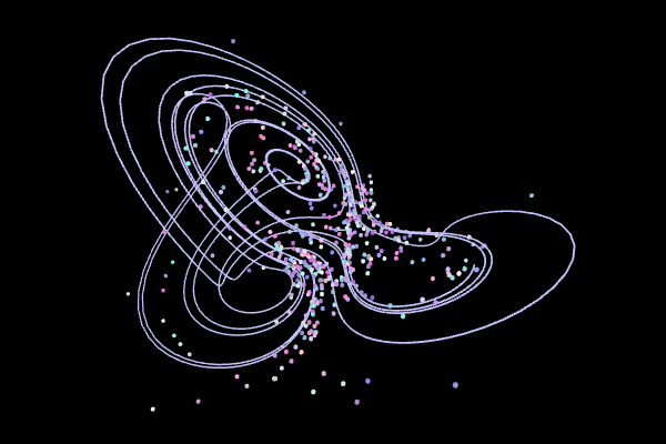
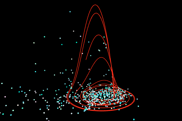
Lorenz83
Parameters:
$a = 0.95,$ $b = 7.91,$ $f = 4.83,$ $g = 4.66$
System:
$\left\{ \begin{eqnarray*} \frac{dx}{dt}&=&-a x - y^2 - z^2 + a f\\ \frac{dy}{dt}&=& -y + x y - b x z + g\\ \frac{dz}{dt}&=& -z + b x y + x z \end{eqnarray*}\right. $
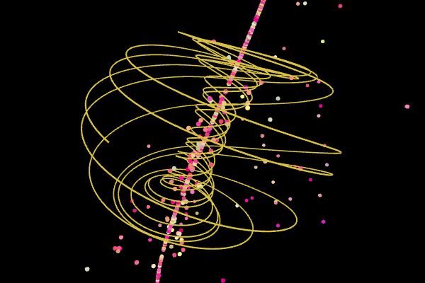
Rössler
Parameters:
$a = 0.2$, $b = 0.2$, $c = 5.7$
System:
$\left\{ \begin{eqnarray*} \frac{dx}{dt}&=&-(y+z)\\ \frac{dy}{dt}&=&x+ay\\ \frac{dz}{dt}&=&b+z(x-c) \end{eqnarray*}\right. $
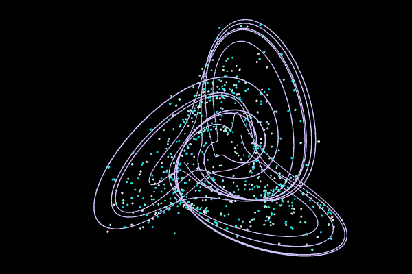
Halvorsen
Parameter:
$a = 1.89$
System:
$\left\{ \begin{eqnarray*} \frac{dx}{dt}&=&-a x-4y-4z-y^2 \\ \frac{dy}{dt}&=& -a y-4z-4x-z^2 \\ \frac{dz}{dt}&=& -a z-4x-4y-x^2 \end{eqnarray*}\right. $
Rabinovich-Fabrikant
Parameters:
$\alpha = 0.14$, $\gamma = 0.10$
System:
$\left\{ \begin{eqnarray*} \frac{dx}{dt}&=&y ( z - 1 + x^2 ) + \gamma x\\ \frac{dy}{dt}&=&x ( 3 z + 1 - x^2 ) + \gamma y\\ \frac{dz}{dt}&=& - 2 z ( \alpha + x y ) \end{eqnarray*}\right. $
Three-Scroll Unified Chaotic System
Parameters:
$a = 32.48,$ $b = 45.84,$ $c = 1.18,$
$d = 0.13,$ $e = 0.57$, $f = 14.7$
System:
$\left\{ \begin{eqnarray*} \frac{dx}{dt}&=&a(y-x)+d x z \\ \frac{dy}{dt}&=& bx-x z + f y \\ \frac{dz}{dt}&=& cz+xy-ex^2 \end{eqnarray*}\right. $
Sprott
Parameters:
$a = 2.07$, $b = 1.79$
System:
$\left\{ \begin{eqnarray*} \frac{dx}{dt}&=& y + a x y +x z \\ \frac{dy}{dt}&=& 1 - b x^2 +yz \\ \frac{dz}{dt}&=& x-x^2-y^2 \end{eqnarray*}\right. $
Four-Wing
Parameters:
$a = 0.2,$ $b = 0.01,$ $c = -0.4$
System
$\left\{ \begin{eqnarray*} \frac{dx}{dt}&=& ax+yz \\ \frac{dy}{dt}&=& b x + cy - xz \\ \frac{dz}{dt}&=& -z-xy \end{eqnarray*}\right. $
The source code can be found here. For the 3d enviroment I used the p5.EasyCam library developed by Thomas Diewald. I used the dat.GUI library for the controls. The position of a particle is computed with a 4th order Runge-Kutta method.
Finally, if you find this content useful, please consider supporting my work using the links below.
I sincerely appreciate it. Thank you! 😃

References
- Aizawa, Y. (1982). Global Aspects of the Dissipative Dynamical Systems I: Statistical Identification and Fractal Properties of the Lorenz Chaos. Progress Theoret Physics. 68(1):64-84.
- Aizawa, Y. (1982). Global Aspects of the Dissipative Dynamical Systems II: Periodic and Chaotic Responses in the Forced Lorenz System Progress Theoret Physics. 68(6):1864-1879.
- Dadras, S., Momeni, H.R. (2009). A novel three-dimensional autonomous chaotic system generating two, three and four-scroll attractors. Physics Letters A. Volume 373, Issue 40. pp. 3637-3642.
- Langford, W. F. (1984). Numerical studies of torus bifurcations, Numerical methods for bifurcation problems (Dortmund, 1983), Internat. Schriftenreihe Numer. Math., vol. 70, Birkhäuser, Basel, pp. 285-295.
- Lorenz E. N. (1963). Deterministic Nonperiodic Flow. Journal of the Atmospheric Sciences. 20(2): 130–141.
- Lorenz E. N. (1993). The Essence of Chaos University of Washington Press.
- Lucas, S. K., Sander, E. & Tallman, L. (2020). Modeling Dynamical Systems for 3D Printing. Notices of the AMS. 67(11). pp. 1692-1702.
- Pan, L., Zhou, W., Fang,J., Li, D. (2010). A new three-scroll unified chaotic system coined. International Journal of Nonlinear Science. vol. 10, 462-474.
- Rössler, O. E. (1976). An Equation for Continuous Chaos. Physics Letters, 57A (5): 397–398.
- Ruelle, D. & Takens, F. (1971). On the Nature of Turbulence. Communications in Mathematical Physics. 20. 167-192.
- Schuster, H. G. (1989). Deterministic Chaos. VCH.
- Solís Pérez, J. E., Gómez-Aguilar, J. F., Baleanu, D., Tchier, F. (2018). Chaotic Attractors with Fractional Conformable Derivatives in the Liouville–Caputo Sense and Its Dynamical Behaviors. Entropy. 2018, 20(5), 384.
- Sprott. J. C. (2014). A dynamical system with a strange attractor and invariant tori. Physic Letters A, 378 1361-1363.
- Strogatz, S. H. (2018). Nonlinear Dynamics and Chaos. CRC Press.
- Thomas, René. (1999). Deterministic chaos seen in terms of feedback circuits: Analysis, synthesis, ‘labyrinth chaos’. Int. J. Bifurcation and Chaos. 9 (10): 1889–1905.
- Tam L., Chen J., Chen H., Tou W. (2008). Generation of hyperchaos from the Chen–Lee system via sinusoidal perturbation. Chaos, Solitons and Fractals. Vol. 38, 826-839.
- Wang, Z., Sun, Y., van Wyk, J. B, Qi, G, van Wyk, M. A. (2009). A 3-D four-wing attractor and its analysis. Brazilian Journal of Physics, vol. 39, no. 3. pp.547-553.